Milestone 2 Report
Reports ·Develop framework for the hybrid models identifying the known and unknown parts along with mathematical approaches.
In the first milestone report we identified the components of our deep learning model for the prediction of tipping points in the climate system. We also identified appropriate training datasets to train the CNN. Much of this work was to facilitate the inclusion of spatially explicit datasets to expand our ability to detect EWS beyond temporal datasets and exploit the additional information provided by the two additional dimensions in spatial data. Here, we explain further developments to the framework for our CNN and explore data sets that we have used for training and for model performance testing. We have identified additional datasets to be included in our training set, as well as situations where the CNN is challenged. We suggest ways to improve upon the CNN performance.
Develop framework for the hybrid model
We have developed a framework to expand the CNN to work with spatial data and phase transitions as well as bifurcations. While bifurcations can occur on low-dimensional manifolds in climate systems, this is not the only mechanism by which abrupt transitions might take place. Higher-dimensional, spatially organized systems admit discontinuous shifts of equilibrium that are described by the theoretical framework of phase transitions. These phenomena bear some relationship to dynamical bifurcations (in some cases mean-field approximations provide a reduced form for a system undergoing a phase transition which is equivalent to the normal form for a known bifurcation). However, phase transitions can be more varied in their manifestation and produce different early warning signals leading up to a transition. This added diversity will require a more sophisticated model to successfully classify time series data, but may offer a tool that is much more generalizable and robust to false positives than the simpler ODE bifurcation model. Recent theoretical work supports the hypothesis that early warning signal detection in the phase transition framework may present the opportunity to leverage more modern, data-intensive computational techniques to improve performance1, which is our goal with this neural model.
We have developed a framework to expand the CNN to work with spatial data and phase transitions as well as bifurcations. While bifurcations can occur on low-dimensional manifolds in climate systems, this is not the only mechanism by which abrupt transitions might take place. Higher-dimensional, spatially organized systems admit discontinuous shifts of equilibrium that are described by the theoretical framework of phase transitions. These phenomena bear some relationship to dynamical bifurcations (in some cases mean-field approximations provide a reduced form for a system undergoing a phase transition which is equivalent to the normal form for a known bifurcation). However, phase transitions can be more varied in their manifestation and produce different early warning signals leading up to a transition. This added diversity will require a more sophisticated model to successfully classify time series data, but may offer a tool that is much more generalizable and robust to false positives than the simpler ODE bifurcation model. Recent theoretical work supports the hypothesis that early warning signal detection in the phase transition framework may present the opportunity to leverage more modern, data-intensive computational techniques to improve performance, which is our goal with this neural model.
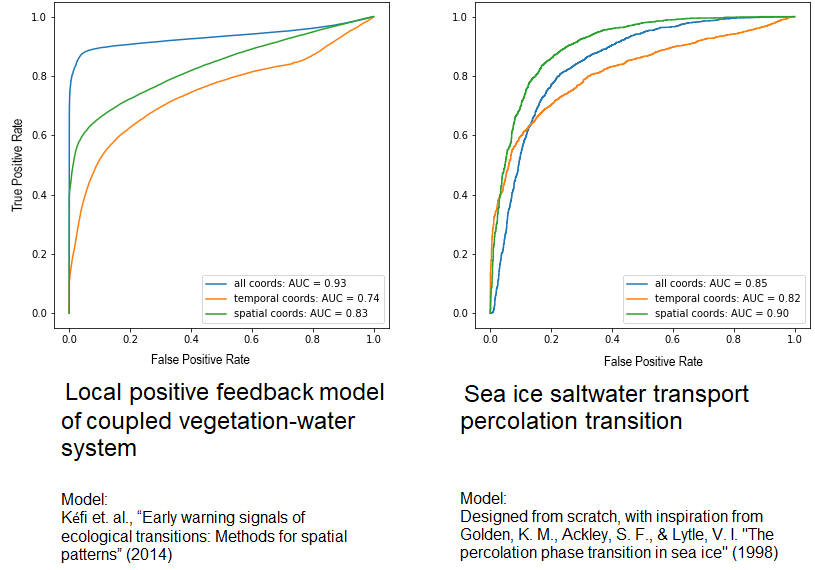
Results from our prototype model on some simulated datasets have been promising. Tested on a withheld portion of the training set, the CNN-LSTM correctly classifies more than 95% of runs from first-order transition models and more than 99% of those of second order, even when it is supplied with time series data truncated well before the observed transition. We have also tested it on simulated data from non-Ising systems undergoing phase transitions: a coupled vegetation-water system which undergoes an aridification transition as rainfall decreases, and a simple sea ice model which exhibits a percolation phase transition in saltwater content as its porosity increases. ROC curves for the model’s true- vs. false-positive classification rates at varied discrimination thresholds are plotted above. For both systems, the model trained exclusively on Ising model data transfers quite well to the new test case (area under ROC curve ≥ 85%). Results are presented for models trained on only spatial or only temporal EWS statistics (green, orange) as well as those trained on all statistics together (blue). Interestingly, classification of the sea ice percolation transitions is more successful when the temporal information is omitted entirely. We suspect that while theory suggests that EWS information should be present in all of these coordinates, the specific dynamical properties and characteristic time- and length-scales of a given system may render one set of statistics more useful than another. Preliminary tests on climate data for abrupt transitions identified in CMIP5 simulations have yielded mixed results; on some models in the repository the classifier performs quite well (area under ROC curve up to 93%), but on others its performance is less impressive (AUC near 50%). There is, however, no guarantee that the transitions in this data set originate from dynamical phase transitions, so it is difficult to evaluate the classifier based on these results.
Identification of the known and unknown parts
Moving forward, we hope to more thoroughly explore options to augment and diversify our training data set. Our approach is premised on the predicted universality of early warning signals leading up to transitions, which enables a model trained on simple synthetic data to transfer to empirical climate data. However, with ODE bifurcation data and even more so with spatiotemporal phase transition data, there is substantial variety to how abrupt transitions might manifest and it remains an open question how diverse our training set needs to be to transfer to an arbitrary transition event. Phase transitions can be classified as first- or second-order, the former of which is less theoretically well-described with respect to the expected presentation of early warning signals. Phase transitions are also often categorized into universality classes based on critical exponents of their power-law behavior close to the critical point, but these are typically governed by dimensionality and spatial and lattice symmetries of the system, and it is not clear to what extent this might provide insight into transfer properties to real climate data. Practically speaking, we plan to approach this problem by implementing a larger variety of phase transition models and systematically determining which ones most improve the model’s performance on data from other, withheld systems. We hope to observe asymptotic behavior in classification accuracy as more training examples are introduced, which would provide an indirect indication that the model has attained near-universal generalizability to a wide range of transition events. We will also explore whether accuracy can be improved by merging training sets derived from phase transition models with sets derived from climate-specific models (for instance by using data augmentation on CMIP5 output time series).
We have highlighted the collapse of the Atlantic Meridional Overturning Circulation (AMOC) as a case study to test the deep learning (DL) approach on, using output from a low-resolution GCM that has been forced to exhibit the collapse2. Our previous work has shown that generic early warning signals (EWS; increasing AR(1) and variance) can be found with varying degrees of success depending on the latitude of the overturning strength3. The DL method detects the collapse most readily in similar latitudes to the generic EWS. However it is unable to decide what the most likely bifurcation the system is approaching; it can clearly detect that it is not a Hopf bifurcation, but at certain latitudes it suggests it is a fold, and others a transcritical. The hysteresis behavior in the model leads us to believe it is a fold and that the higher complexity of the model is creating confusion for the DL method. However, recent studies suggest that it may be another mechanism altogether that will cause tipping of the AMOC called multifrequency tipping which is tipping due to the disappearance of an attracting torus4. It is also confused by equilibrium runs of the same GCM (where the forcing causing the collapse is increased and then held constant, allowing the system to settle to some equilibrium). Generic EWS can determine that there is no movement towards collapse but the DL still suggests there is. This may be because despite using the end of these runs for testing, there are long term dynamics that the DL is detecting that are an artifact of the forcing part of these runs. Further analysis is needed regarding these equilibrium runs. We are also exploring the use of a simple 4-box model of AMOC collapse to be used as a training set for the DL, this is able to reproduce AMOC collapse5 well enough to explore how the overturning is affected by varying a number of parameters.
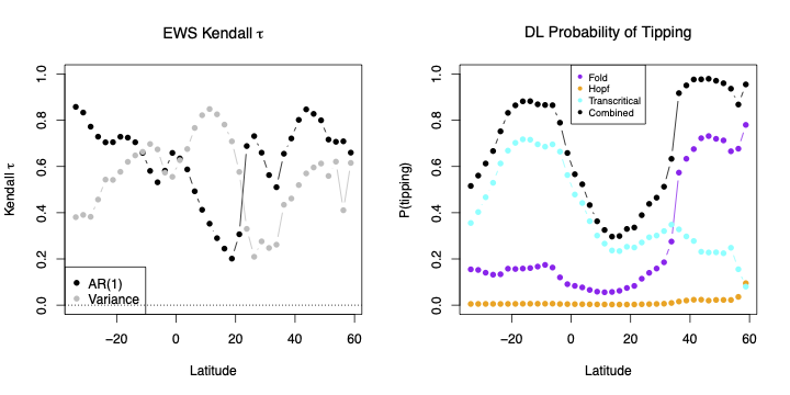 The spatial distribution of where the clearest early warning signals of the approach towards AMOC collapse are observed, matches reasonably well with the latitudes that show the highest probability of collapse according to the deep learning (DL) method. The DL method switches its belief in the type of bifurcation being approached depending on latitude.
We have identified a collection of abrupt shifts in CMIP5 models in the literature6. Of these 30 abrupt shifts, 20 represent rapid changes to a new state, while the others consist of gradual changes, forced transitions and oscillatory switches between two different states. Most of these shifts relate to the cryosphere, with a limited number identified in vegetation systems. The shifts classified as ‘rapid changes to a new state’ present the most applicable dataset, however all classes may prove to be useful. Work has begun to isolate the 1D time series for these shifts to serve as either training data or to test the model on. Further to this, exploring higher dimensional model data around these shifts will provide further information to train the machine learning algorithm on.
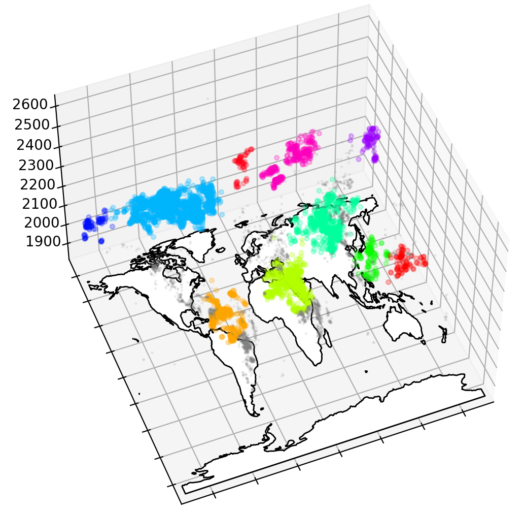 The analytical pipeline detects abrupt shifts in grid cell time series and then clusters these grid cells both in space, and in time based on when the shift occurred. The results show abrupt shifts in vegetation carbon and sea ice in output from the LPJmL land surface model and PISM [Image credit: Sina Loriani, Potsdam Institute for Climate Impact Research]
We have also found further examples of abrupt shift detection in CMIP5 models7. This provides a methodology for the automation of abrupt shift identification using edge detection in multiple dimensions (2D with a time component). These spatio-temporal shifts have been identified in a majority of CMIP5 models and are likely to prove useful in training or testing our deep learning approach. We have also continued development - in collaboration with Potsdam Institute for Climate Impact Research - on an analytical pipeline to automatically detect potential tipping points in space and time and will use this to detect tipping points in CMIP5 and CMIP6 data. Currently, this is still under development and the initial tests are on abrupt shifts in vegetation carbon from running the LPJmL land surface model under RCP8.5 climate forcing from HADGEM and abrupt shifts in sea ice from output from PISM (see above figure for example of spatio-temporal clustering). The 2D spatio-temporal representation for these identified tipping points can be used to test or train the phase transition model.
-
Hagstrom, G., & Levin, S. I. (2021). Phase transitions and the theory of early warning indicators for critical transitions. Global Systemic Risk, 1–16. ↩
-
Hawkins, E., Smith, R. S., Allison, L. C., Gregory, J. M., Woollings, T. J., Pohlmann, H., & De Cuevas, B. (2011). Bistability of the Atlantic overturning circulation in a global climate model and links to ocean freshwater transport. Geophysical Research Letters, 38(10). ↩
-
Boulton, C.A., Allison, L.C. and Lenton, T.M., (2014). Early warning signals of Atlantic Meridional Overturning Circulation collapse in a fully coupled climate model. Nature communications, 5(1), pp.1-9. ↩
-
Keane, A., Krauskopf, B., & Lenton, T. M. (2020). Signatures consistent with multifrequency tipping in the atlantic meridional overturning circulation. Physical Review Letters, 125(22), 228701. ↩
-
Gnanadesikan, A., Kelson, R. and Sten, M., (2018). Flux correction and overturning stability: Insights from a dynamical box model. Journal of Climate, 31(22), pp.9335-9350. ↩
-
Drijfhout, S., Bathiany, S., Beaulieu, C., Brovkin, V., Claussen, M., Huntingford, C., Scheffer, M., Sgubin, G. and Swingedouw, D., (2015). Catalogue of abrupt shifts in Intergovernmental Panel on Climate Change climate models. Proceedings of the National Academy of Sciences, 112(43), pp.E5777-E5786. ↩
-
Bathiany, S., Hidding, J. and Scheffer, M., (2020). Edge detection reveals abrupt and extreme climate events. Journal of Climate, 33(15), pp.6399-6421. ↩